Panel Fixed Effects for Causal Inference#

Suppose we want to estimate the effect of a training program on earnings. Workers who take it may be more motivated or able to begin with. If we simply compare trained vs untrained workers, we mix the program effect with that pre-existing difference—our estimate is confounded. Panel data (the same units observed over time) and fixed effects let us control for such time-invariant differences by comparing each unit to itself. This notebook shows when that works, when it fails, and how to do it in CausalPy.

Panel data tracks the same units (workers, firms, countries) over multiple time periods. Fixed effects exploits this structure to control for unobserved confounders—either unit-specific characteristics, common time shocks, or both.

Unit-specific characteristics are traits that differ across units but are roughly stable over time for each unit. They can be observed (e.g., industry, region) or unobserved (e.g., managerial talent, culture). Examples by setting:

Workers: innate ability, motivation, risk tolerance, education (if unchanging in the panel).
Firms: management quality, corporate culture, brand strength, baseline productivity.
Regions or countries: institutions, legal tradition, geography, norms.

Common time shocks are events or conditions at a given time that affect all units in the panel in a similar way (even if intensity varies). Examples:

Macroeconomic: recessions, interest-rate cycles, commodity price spikes, exchange-rate moves.
Policy: a nationwide minimum-wage change, a new regulation, or a tax reform that applies to all units.
Technology or information: adoption of a new technology, a widely publicized health finding, or a common demand shock (e.g., pandemic).

Note

Why this matters for causal inference. If treatment assignment is correlated with unit-level traits (e.g., better firms adopt the policy first) or with common time shocks (e.g., treatment rolls out in a recession), naive comparisons are confounded. Fixed effects remove the part of the variation in the outcome that is explained by unit dummies (unit FE), time dummies (time FE), or both, so we can isolate the effect of treatment.

Roadmap. We first set up the confounding problem and the fixed-effects toolbox (dummies vs demeaned). Then we work through four examples: one-way unit FE (simulation with known truth), when FE fails (time-varying confounder), two-way FE (state–year policy), and large-panel demeaned (workers × waves). We end with when to use FE, how to choose unit/time/two-way, and limitations.

Two ways to implement fixed effects. We can control for unit (or time) effects in either of two equivalent ways: (1) dummy variables (unpooled FE)—include a separate intercept for each unit and/or time period—or (2) demeaned transformation—subtract from each variable its mean within the group (e.g. within unit). Demeaning removes any part of the outcome that is constant within that group (such as \(u_i\) within unit \(i\)), so we get the same causal estimate without estimating hundreds of nuisance parameters. We’ll use both approaches in the examples below so you see that they give identical results.

This notebook focuses on these two fixed-effects implementations. Hierarchical/partial-pooling panel models are a different approach and are out of scope here.

For a deeper treatment of panel data methods and causal inference, see Cunningham [2021] (Chapter 8), Huntington-Klein [2021], and Wooldridge [2010].

import warnings

import matplotlib.pyplot as plt
import numpy as np
import pandas as pd
import seaborn as sns
from sklearn.linear_model import LinearRegression

import causalpy as cp

warnings.filterwarnings("ignore")

%config InlineBackend.figure_format = 'retina'
plt.style.use("default")

%load_ext autoreload
%autoreload 2

# Figure sizing (consistent width for all figures; multiply height only when needed)
FIG_WIDTH = 10
FIG_HEIGHT = 5

# Sampling settings for Bayesian models
sample_kwargs = {
    "draws": 2000,
    "tune": 1000,
    "chains": 4,
    "target_accept": 0.95,
    "random_seed": 42,
}

The Confounding Problem#

The standard panel data model is:

\[y_{it} = \beta D_{it} + u_i + \gamma_t + \epsilon_{it}\]

where \(D_{it}\) is treatment and \(\epsilon_{it}\) is idiosyncratic error. The terms \(u_i\) and \(\gamma_t\) are nuisance parameters we must account for to get an unbiased estimate of the causal effect \(\beta\):

\(u_i\) captures everything about unit \(i\) that is constant over time but affects the outcome (e.g., a worker’s innate ability, a firm’s culture). There is one \(u_i\) parameter per unit.
\(\gamma_t\) captures shocks at time \(t\) that affect all units equally (e.g., a recession, a policy change). There is one \(\gamma_t\) parameter per time period.

These become confounders if they also influence treatment assignment:

Confounder	What it is	Example	Solution
\(u_i\) (unit effect)	Time-invariant unit characteristics	Worker ability, firm culture	Unit FE
\(\gamma_t\) (time effect)	Common shocks affecting all units	Recessions, policy changes	Time FE

Without accounting for these, any correlation between \(D_{it}\) and \(u_i\) or \(\gamma_t\) biases our estimate. The DAG below illustrates both confounding paths:

../_images/76030549f0e4637d54e45327de652afe9b195f2382887775f8cac360bee79cff.svg

Figure (DAG). Nodes: \(u_i\) (unit effect) and \(\gamma_t\) (time effect), unobserved, dashed ellipses; \(D_{it}\) (treatment), \(Y_{it}\) (outcome). Red dashed edges: unit confounding paths (\(u_i \to D\), \(u_i \to Y\)). Blue dashed edges: time confounding paths (\(\gamma_t \to D\), \(\gamma_t \to Y\)). Solid black edge: causal effect \(\beta\).

In summary, estimating the causal effect of treatment on the outcome risks bias from time-invariant unit effects, common temporal shocks, or both [Imai and Kim, 2019]. These confounders create backdoor paths. Normally we would close backdoor paths by conditioning, but we can’t do that directly here because they are unobserved. However, because these confounders have a specific structure (constant within units or across units), adding fixed effects can effectively close these backdoor paths.

The Fixed Effects Toolbox#

Fixed effects controls for confounders by comparing units to themselves (unit FE) or comparing across units within the same time period (time FE).

Dummy variables (unpooled FE) vs demeaned transformation. We can implement this either by including a dummy (intercept) for each unit and/or time period, or by demeaning: subtract from each variable its average within the group. For example, to remove unit effects we subtract the unit mean—for unit \(i\), \(\bar{y}_{i\cdot}\) is the average of \(y_{it}\) over time. Anything constant within the unit (including \(u_i\)) then drops out (\(u_i - \bar{u}_{i\cdot} = 0\)), so we don’t need to estimate it. The same idea applies to time: subtract the period mean to remove \(\gamma_t\). Both approaches give the same treatment-effect estimate; we use both in the examples so you can see that, and we prefer demeaning when there are many units or periods to avoid estimating hundreds of coefficients.

Scope note. In this notebook and in PanelRegression for this PR, “dummy variables” means unpooled fixed effects (one coefficient per unit/time category). Hierarchical/partial-pooling panel models are a separate approach and are not implemented here.

Formulas. One-way (unit) demeaning: \(\tilde{y}_{it} = y_{it} - \bar{y}_{i\cdot}\). Two-way (unit and time): \(\tilde{y}_{it} = y_{it} - \bar{y}_{i\cdot} - \bar{y}_{\cdot t} + \bar{y}_{\cdot\cdot}\). The two-way formula is equivalent to the dummy-variable approach for balanced panels.

FE Type	Controls for
Unit FE	\(u_i\) - time-invariant unit characteristics
Time FE	\(\gamma_t\) - common shocks affecting all units
Two-way FE	Both \(u_i\) and \(\gamma_t\)

Key assumptions for fixed effects to identify causal effects [Imai and Kim, 2019]:

Strict exogeneity: No feedback from past outcomes to current treatment
No time-varying confounders: Only time-invariant confounders exist (the key limitation!)
Treatment varies within units: Need some units to change treatment status over time
Parallel trends (for two-way FE): Connects to difference-in-differences assumptions

Example 1: One-Way Fixed Effects (Unit Only)#

This example demonstrates one-way unit fixed effects—we control for time-invariant unit characteristics but NOT for common time trends.

When is this appropriate?

Time trends are not a major concern (no common shocks affecting all units)
Or time effects are captured by covariates in the model
You want to preserve cross-sectional variation that time FE would remove

Data-generating process (DGP). The simulated data are built to match the model \(y_{it} = \beta D_{it} + u_i + \gamma_t + \epsilon_{it}\) with a known \(\beta\):

Unit confounder \(u_i\): Yes. Each unit has a time-invariant draw \(u_i\) that shifts the outcome. Treatment is assigned to the first half of units from period 10 onward, so treatment is correlated with unit identity—and therefore with \(u_i\). That creates confounding: naive OLS will be biased.
Time confounder \(\gamma_t\): No. We do not add any common period shock in this simulation, so there is no time-level confounding. One-way unit FE is the appropriate control; we add time FE later only to show it leaves the estimate unchanged when there is no \(\gamma_t\).

This example is designed to satisfy all the identifying assumptions:

✅ Time-invariant confounders only (unit effects \(u_i\))
✅ No feedback from outcomes to treatment
✅ No time-varying confounders
✅ Treatment varies within units over time

Causal question: What is the effect of treatment on the outcome, controlling for unobserved unit-level heterogeneity?

# Set up random number generator
rng = np.random.default_rng(42)

# Panel dimensions
n_units = 20
n_periods = 15
treatment_time = 10

# True parameters
TRUE_TREATMENT_EFFECT = 3.0
TRUE_X_COEF = 0.5

# Generate panel data: y_it = β*D_it + u_i + 0*t + ε_it (no γ_t in this example)
data = []
for i in range(n_units):
    unit_effect = rng.normal(scale=2.0)  # Unit confounder u_i (time-invariant)

    for t in range(n_periods):
        x1 = rng.normal()
        # First half of units get treated after treatment_time → D correlated with unit (hence u_i)
        treatment = 1 if (t >= treatment_time and i < n_units // 2) else 0

        y = (
            unit_effect
            + TRUE_TREATMENT_EFFECT * treatment
            + TRUE_X_COEF * x1
            + rng.normal(scale=0.5)
        )
        # No γ_t term: no time confounder in this DGP

        data.append(
            {
                "unit": f"unit_{i}",
                "time": t,
                "treatment": treatment,
                "x1": x1,
                "y": y,
            }
        )

df_sim = pd.DataFrame(data)
print(f"Panel: {n_units} units, {n_periods} periods")
print(f"True treatment effect: {TRUE_TREATMENT_EFFECT}")
df_sim.head()

Panel: 20 units, 15 periods
True treatment effect: 3.0

	unit	time	x1	y
0	unit_0	0	-1.039984	0.464668
1	unit_0	1	0.940565	0.104199
2	unit_0	2	-1.302180	0.022265
3	unit_0	3	-0.316243	0.442912
4	unit_0	4	-0.853044	0.622611

../_images/a714589bb308d80a6feb5efac57a78b56e9d84b7267cc50d1efd0e150f964c5e.png

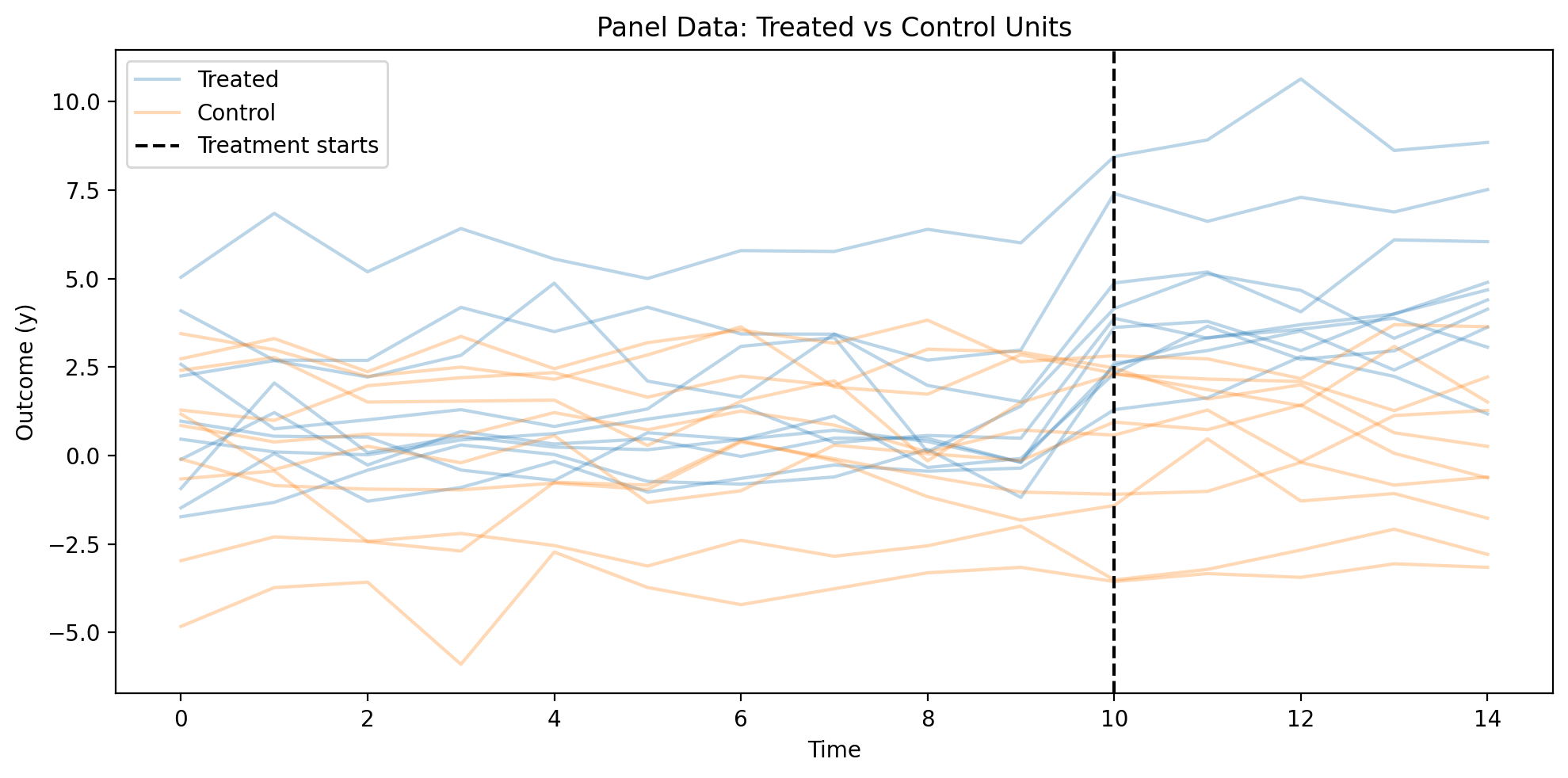
Figure (Example 1). Outcome \(y\) by time (periods 0–14); one line per unit, grouped by treated vs control. Vertical black dashed line: treatment start (\(t = 10\)). True treatment effect in the DGP is \(\beta = 3\).

Naive OLS (Biased)#

First, let’s see what happens if we ignore the unit fixed effects:

# Naive OLS without fixed effects
X_naive = df_sim[["treatment", "x1"]].values
y_naive = df_sim["y"].values

naive_model = LinearRegression().fit(X_naive, y_naive)
print("Naive OLS (NO fixed effects):")
print(f"  Treatment effect: {naive_model.coef_[0]:.3f} (True: {TRUE_TREATMENT_EFFECT})")
print(f"  Bias: {naive_model.coef_[0] - TRUE_TREATMENT_EFFECT:.3f}")

Naive OLS (NO fixed effects):
  Treatment effect: 3.796 (True: 3.0)
  Bias: 0.796

Fixed Effects with Dummies#

# One-way unit FE with dummy variables (Bayesian)
# Note: time_fe_variable is not set, so we only control for unit effects
result_dummies = cp.PanelRegression(
    data=df_sim,
    formula="y ~ C(unit) + treatment + x1",  # No C(time) - unit FE only
    unit_fe_variable="unit",
    fe_method="dummies",
    model=cp.pymc_models.LinearRegression(sample_kwargs=sample_kwargs),
)

result_dummies.summary()

Panel Regression
============================================================
Units: 20 (unit)
FE method: dummies
Observations: 300
============================================================

Note: 19 fixed effect coefficients not shown (use print_coefficients() to see all)

Model Coefficients:
Model coefficients:
    Intercept    0.75, 94% HDI [0.49, 1]
    treatment    3.1, 94% HDI [2.9, 3.3]
    x1           0.5, 94% HDI [0.44, 0.56]
    y_hat_sigma  0.51, 94% HDI [0.47, 0.56]

The treatment effect estimate (treatment 3.1, 94% HDI [2.9, 3.3]) closely recovers the true value of 3.0, and the 94% HDI contains the true parameter. This demonstrates that one-way unit fixed effects successfully removes the bias from time-invariant unit confounders \(u_i\).

Same estimate via demeaned transformation#

We now use the demeaned transformation (introduced in the Toolbox): subtract each variable’s mean within the unit. No unit dummies in the formula—the transformation handles it. The estimate is identical:

# One-way unit FE with demeaned transformation (Bayesian)
# Note: time_fe_variable is not set, so we only control for unit effects
result_demeaned = cp.PanelRegression(
    data=df_sim,
    formula="y ~ treatment + x1",  # No C(unit) needed with demeaned transformation!
    unit_fe_variable="unit",
    # time_fe_variable not set = one-way unit FE
    fe_method="demeaned",
    model=cp.pymc_models.LinearRegression(sample_kwargs=sample_kwargs),
)

result_demeaned.summary()

Panel Regression
============================================================
Units: 20 (unit)
FE method: demeaned
Observations: 300
============================================================

Model Coefficients:
Model coefficients:
    Intercept    1.1e-05, 94% HDI [-0.054, 0.053]
    treatment    3.1, 94% HDI [3, 3.3]
    x1           0.5, 94% HDI [0.44, 0.56]
    y_hat_sigma  0.5, 94% HDI [0.46, 0.54]

Interpreting the Results#

The treatment coefficient of approximately 3.1 (true value: 3.0) represents the within-unit causal effect of treatment on the outcome.

What this means: For the same unit, receiving treatment increases the outcome by about 3 units on average, after controlling for all time-invariant unit characteristics.

Key insight: This estimate comes from comparing each unit to itself at different time points - not from comparing treated units to control units. This is why fixed effects can control for unobserved unit-level confounders.

The Bayesian credible interval provides uncertainty quantification: we’re 94% confident the true effect lies within this range.

Comparing One-Way vs Two-Way Fixed Effects#

Recall that our simulated data includes unit-specific confounders (\(u_i\)) but no common time shocks (\(\gamma_t\)) that affect all units equally. What happens if we add time fixed effects anyway? Let’s compare:

One-way (unit only): What we just estimated above
Two-way (unit + time): Adding time fixed effects

Since there are no time shocks in this data, we expect both estimates to be similar. This illustrates that adding unnecessary fixed effects doesn’t bias estimates—but it does consume degrees of freedom.

# Two-way FE: Add time fixed effects to the same data
result_twoway = cp.PanelRegression(
    data=df_sim,
    formula="y ~ treatment + x1",  # Demeaned transformation handles both unit and time
    unit_fe_variable="unit",
    time_fe_variable="time",  # <-- This adds time FE!
    fe_method="demeaned",
    model=cp.pymc_models.LinearRegression(sample_kwargs=sample_kwargs),
)

# Compare the treatment effect estimates
print("=" * 60)
print("COMPARISON: One-Way vs Two-Way Fixed Effects")
print("=" * 60)
print(f"\nTrue treatment effect: 3.0")
print(f"\nOne-way (unit FE only):")
print(
    f"  Treatment coefficient: {result_demeaned.model.idata.posterior['beta'].sel(coeffs='treatment').mean().values:.3f}"
)
print(f"\nTwo-way (unit + time FE):")
print(
    f"  Treatment coefficient: {result_twoway.model.idata.posterior['beta'].sel(coeffs='treatment').mean().values:.3f}"
)
print("\nIn this case, both estimates are similar because the simulated data")
print("doesn't have strong common time trends that confound treatment.")

============================================================
COMPARISON: One-Way vs Two-Way Fixed Effects
============================================================

True treatment effect: 3.0

One-way (unit FE only):
  Treatment coefficient: 3.120

Two-way (unit + time FE):
  Treatment coefficient: 3.071

In this case, both estimates are similar because the simulated data
doesn't have strong common time trends that confound treatment.

Tip

When does the choice matter?

The estimates from one-way and two-way FE will differ when:

There are common time shocks (e.g., a recession affecting all units) that correlate with treatment
Treatment rollout is correlated with time trends (e.g., early adopters vs late adopters)

If neither condition applies, one-way unit FE is often sufficient and more parsimonious.

Example 2: When Fixed Effects Fails#

The simulation above worked because our data satisfied all the identifying assumptions. But what happens when those assumptions are violated? We continue with one-way unit fixed effects to isolate the problem.

Here we add a time-varying confounder—an economic shock that varies by unit and time—that affects both treatment and outcome. Workers are more likely to seek training during good economic times, and the shock also directly affects productivity. Unit fixed effects cannot remove this confounder because it changes over time, and time fixed effects cannot remove it either because it varies across units. No combination of fixed effects can eliminate confounders that vary in both dimensions.

# Simulate data with a TIME-VARYING confounder
rng = np.random.default_rng(42)

n_units = 20
n_periods = 15
TRUE_TREATMENT_EFFECT = 3.0  # Same as before

data_violation = []
for i in range(n_units):
    unit_effect = rng.normal(scale=2.0)  # Time-invariant (FE handles this)

    for t in range(n_periods):
        # TIME-VARYING confounder: an economic shock that varies by unit AND time
        economic_shock = rng.normal(scale=1.5)

        # Treatment is AFFECTED by the economic shock (more likely to train during good times)
        treatment_propensity = 0.3 + 0.3 * (economic_shock > 0)
        treatment = 1 if (rng.random() < treatment_propensity and t >= 5) else 0

        # Outcome is affected by treatment AND the economic shock
        y = (
            unit_effect
            + TRUE_TREATMENT_EFFECT * treatment
            + 2.0 * economic_shock  # Direct effect of confounder on outcome
            + rng.normal(scale=0.5)
        )

        data_violation.append(
            {"unit": f"unit_{i}", "time": t, "treatment": treatment, "y": y}
        )

df_violation = pd.DataFrame(data_violation)

# Apply fixed effects
result_violation = cp.PanelRegression(
    data=df_violation,
    formula="y ~ treatment",
    unit_fe_variable="unit",
    fe_method="demeaned",
    model=LinearRegression(),
)

============================================================
FIXED EFFECTS WITH TIME-VARYING CONFOUNDER
============================================================
True treatment effect:      3.00
FE estimate:                3.93
Bias:                       0.93

⚠️  The estimate is BIASED because the economic shock
   affects both treatment and outcome, and FE cannot remove it!
============================================================

../_images/291631a15db51573105dfd565017b899337a2e4373920cc483153545a4fa3c71.png

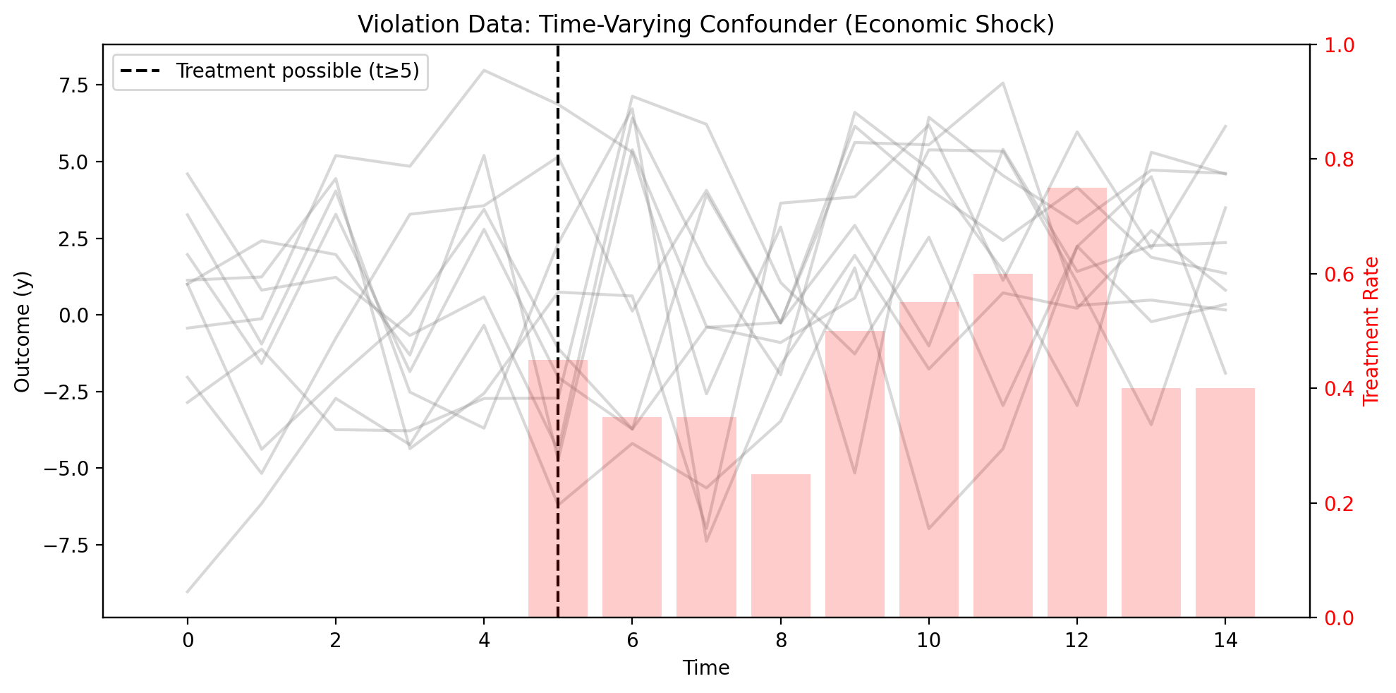
Figure (Example 2). Left axis: outcome \(y\) by time; gray lines = unit-level trajectories. Right axis: treatment rate by period (bars). Vertical black dashed line: first period when treatment is possible (\(t \geq 5\)).

Units experiencing positive economic shocks are both more likely to be treated and have higher outcomes, creating confounding that fixed effects cannot remove.

This example demonstrates a critical limitation: fixed effects only removes time-invariant confounders. In DAG terms, adding a time-varying confounder \(v_{it}\) creates an open backdoor path that fixed effects cannot close:

../_images/bdbdef7e1dac2ee7c5b6d131aaf36781d573d00c5c5553b1b43e75dbcf61e7d1.svg

Fixed effects eliminates the \(u_i\) backdoor path (gray, dashed) but not the \(v_{it}\) path (red). The estimate remains biased.

Important

Before using fixed effects, ask yourself: Are there any unobserved factors that change over time and affect both my treatment and outcome? If yes, fixed effects alone is insufficient.

Connection to Difference-in-Differences#

Two-way fixed effects (TWFE) - with both unit and time fixed effects - is closely related to difference-in-differences (DiD).

With a simple 2x2 design (2 groups, 2 periods, binary treatment), TWFE produces numerically identical estimates to the classic DiD estimator. The model:

\[Y_{it} = \alpha_i + \gamma_t + \beta \cdot D_{it} + \epsilon_{it}\]

where:

\(\alpha_i\) = unit fixed effects
\(\gamma_t\) = time fixed effects
\(D_{it}\) = treatment indicator

is a workhorse of applied causal inference. The coefficient \(\beta\) captures the treatment effect.

With more complex designs (staggered treatment adoption, heterogeneous effects), TWFE and simple DiD can diverge. Recent econometrics research [de Chaisemartin and D'Haultfœuille, 2020] has highlighted that TWFE can give misleading results when:

Treatment effects vary over time (dynamic effects)
Treatment rolls out at different times (staggered adoption)
Treatment effects differ across units (heterogeneity)

For these cases, consider using CausalPy’s DifferenceInDifferences class or newer estimators designed for staggered designs.

Example 3: Two-Way Fixed Effects (Unit + Time)#

When both unit and time confounders matter, we use two-way fixed effects. This example illustrates that with state-level policy data.

Two-way fixed effects (TWFE) is the workhorse model in applied economics and the foundation of difference-in-differences analysis.

Causal Question: What is the effect of a state policy on outcomes, controlling for both state-specific factors and common time trends?

This example uses two-way fixed effects (state + year FE), which controls for:

Time-invariant state characteristics (state FE) — e.g., geography, political culture
Common shocks affecting all states in a given year (year FE) — e.g., national economic conditions

When to use two-way FE:

Treatment timing varies across units (staggered adoption)
Common time shocks could confound the treatment-outcome relationship
You’re doing a difference-in-differences style analysis

For small panels (e.g., 50 US states), we can use the dummy variable approach.

# Simulate state-level data
rng = np.random.default_rng(123)

n_states = 12
n_years = 10
policy_year = 5

state_data = []
for s in range(n_states):
    state_name = f"State_{chr(65 + s)}"
    state_baseline = rng.normal(loc=50, scale=5)

    for y in range(n_years):
        policy = 1 if (y >= policy_year and s < n_states // 2) else 0
        gdp_growth = rng.normal(scale=2)

        outcome = (
            state_baseline
            + 0.3 * y
            + 5.0 * policy
            + 0.5 * gdp_growth
            + rng.normal(scale=1.5)
        )

        state_data.append(
            {
                "state": state_name,
                "year": y,
                "policy": policy,
                "gdp_growth": gdp_growth,
                "outcome": outcome,
            }
        )

df_states = pd.DataFrame(state_data)
print(f"State panel: {n_states} states, {n_years} years")
df_states.head()

State panel: 12 states, 10 years

	state	year	gdp_growth	outcome
0	State_A	0	-0.735573	46.618494
1	State_A	1	0.387949	46.928714
2	State_A	2	1.154208	45.276802
3	State_A	3	1.083904	46.021452
4	State_A	4	-0.644778	46.077755

../_images/3dc0fc02b538de925fd3198c30c02b152b603f4d141db2227185e958c95cc45f.png

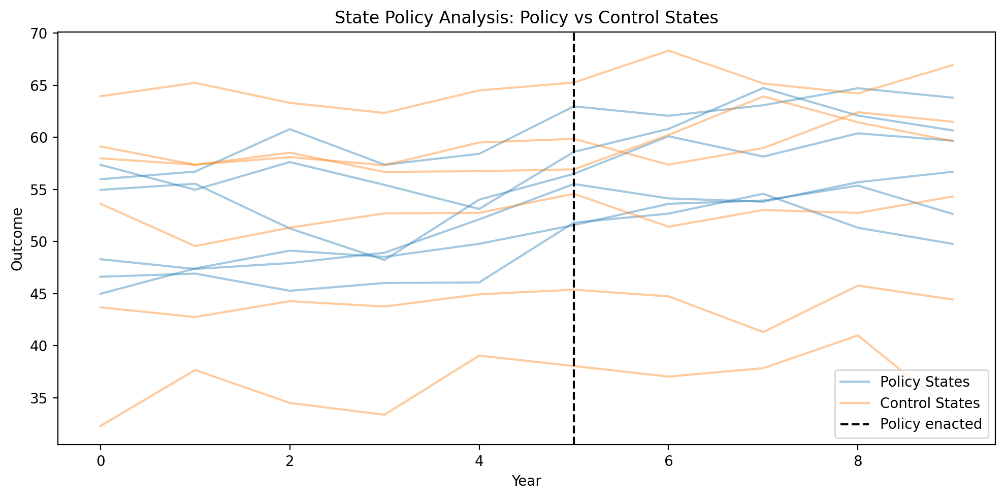
Figure (Example 3). Outcome by year; one line per state, grouped by policy vs control. Vertical black dashed line: policy enactment year. Aggregation by group (policy vs control states).

# Fit panel regression with state and year FE (Bayesian)
result_states = cp.PanelRegression(
    data=df_states,
    formula="outcome ~ C(state) + C(year) + policy + gdp_growth",
    unit_fe_variable="state",
    time_fe_variable="year",
    fe_method="dummies",
    model=cp.pymc_models.LinearRegression(sample_kwargs=sample_kwargs),
)

result_states.summary()

Panel Regression
============================================================
Units: 12 (state)
Periods: 10 (year)
FE method: dummies
Observations: 120
============================================================

Note: 20 fixed effect coefficients not shown (use print_coefficients() to see all)

Model Coefficients:
Model coefficients:
    Intercept    46, 94% HDI [45, 48]
    policy       3.9, 94% HDI [2.9, 5]
    gdp_growth   0.48, 94% HDI [0.33, 0.63]
    y_hat_sigma  1.5, 94% HDI [1.3, 1.7]

# Coefficient plot
# hdi_prob controls the width of the Bayesian HDI interval (default 0.94)
fig, ax = result_states.plot_coefficients(hdi_prob=0.94)
plt.tight_layout()
plt.show()

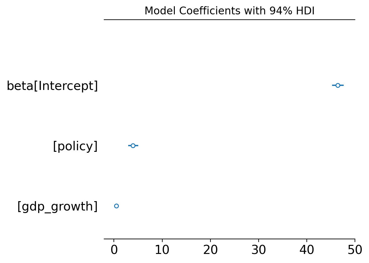
../_images/646accf462f3676542812bf70ce0a0ef1e4c2e218fe576e05244dc41618f627f.png

Figure (coefficients). Posterior distributions of model coefficients (policy, gdp_growth, etc.) with a 94% HDI (highest-density interval) for each parameter’s posterior. You can change the interval width with the hdi_prob argument in plot_coefficients(...) (for example, 0.89 or 0.95). The treatment effect of interest is the policy coefficient.

# Distribution of state fixed effects
fig, ax = result_states.plot_unit_effects()
plt.tight_layout()
plt.show()

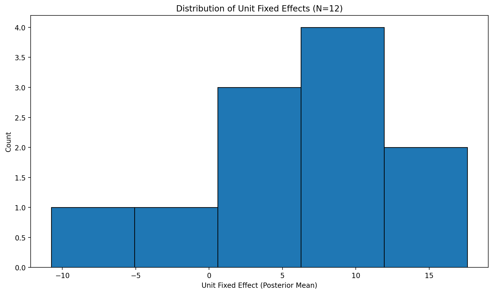
../_images/b7e8becbeecfefea330aa5d813c31b1c48e43eff91577c3902673c7cad8514e4.png

Figure (unit effects). Estimated unit (state) fixed effects: distribution of state-specific intercepts from the two-way FE model.

# State trajectories
# interval_type='mean' shows HDI for the posterior mean (mu), not predictive noise
fig, axes = result_states.plot_trajectories(
    n_sample=6,
    interval_type="mean",
    hdi_prob=0.94,
)
plt.tight_layout()
plt.show()

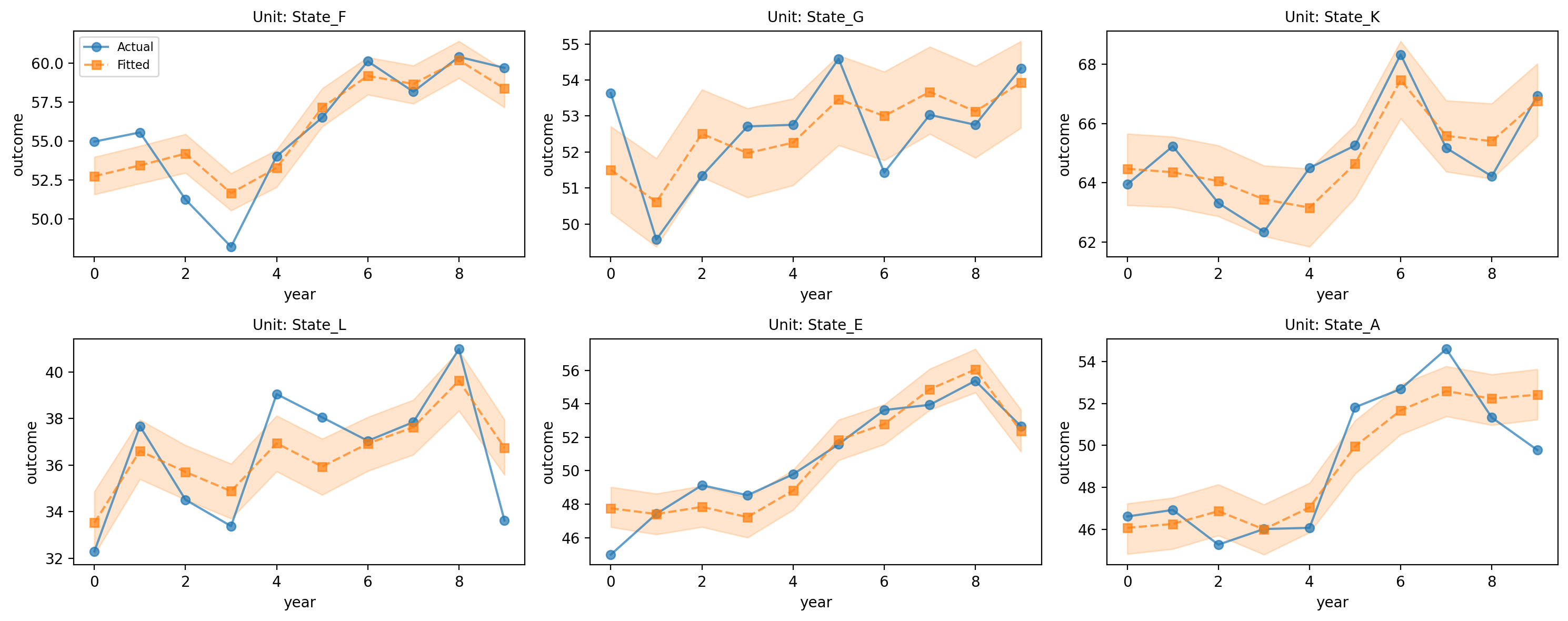
../_images/c5a0ee3fb6a464c4dd0a69a1cbe0d0efe3548589aad182faedc751e2e7a11b51.png

Figure (trajectories). Sample of state-level outcome trajectories; observed vs model (two-way FE). The shaded band is a 94% HDI for the posterior mean trajectory (interval_type="mean"), so it reflects uncertainty in the expected value (mu) rather than full observation noise. Adjust width with hdi_prob in plot_trajectories(...). Used to assess fit and heterogeneity across units.

Example 4: Two-Way FE with Large Panel (Demeaned Transformation)#

With many units, dummy variables don’t scale. We switch to the demeaned transformation and illustrate with a worker panel.

With 200 workers, including dummy variables for each would add 199 coefficients to our model—slow to estimate and cluttering output with nuisance parameters we don’t care about. The demeaned transformation solves this by subtracting group means before estimation, effectively sweeping out the fixed effects without explicitly estimating them.

Causal Question: What is the effect of job training on worker productivity?

This is our motivating example from the introduction! Workers who receive training may differ in unobserved ability - the classic selection problem.

Why two-way FE here?

Worker FE: Controls for innate ability (time-invariant)
Wave FE: Controls for economy-wide conditions affecting all workers

Assumptions we’re making:

Innate ability is time-invariant (plausible)
No time-varying confounders (e.g., no unobserved motivation shocks)
Training doesn’t respond to recent productivity changes

# Simulate worker panel
rng = np.random.default_rng(456)

n_workers = 200
n_waves = 8
training_wave = 4

worker_data = []
for w in range(n_workers):
    worker_id = f"worker_{w:04d}"
    ability = rng.normal(scale=3)

    for wave in range(n_waves):
        trained = 1 if (wave >= training_wave and w < n_workers * 0.4) else 0
        experience = wave * 0.5 + rng.normal(scale=0.2)

        productivity = (
            ability + 2.5 * trained + 0.3 * experience + rng.normal(scale=0.8)
        )

        worker_data.append(
            {
                "worker_id": worker_id,
                "wave": wave,
                "trained": trained,
                "experience": experience,
                "productivity": productivity,
            }
        )

df_workers = pd.DataFrame(worker_data)
print(f"Worker panel: {n_workers} workers, {n_waves} waves")
df_workers.head()

Worker panel: 200 workers, 8 waves

	worker_id	wave	trained	experience	productivity
0	worker_0000	0	0	-0.424790	3.872846
1	worker_0000	1	0	0.492939	0.753789
2	worker_0000	2	0	0.961987	2.445428
3	worker_0000	3	0	1.417059	2.879282
4	worker_0000	4	1	2.389001	6.709637

../_images/62acd557107220b9790d104107e3e1262f66dee503b2e14ca2dea26fe1b44804.png

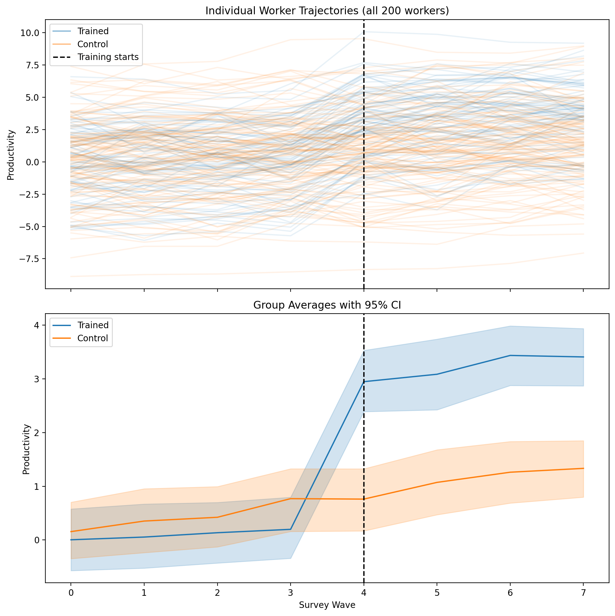
Figure (Example 4). Top: productivity by survey wave, one line per worker (trained vs control). Bottom: group means with 95% CI. Vertical black dashed line: wave when training starts.

# Two-way FE with demeaned transformation (Bayesian)
# Both worker_id and wave are used for fixed effects
result_workers = cp.PanelRegression(
    data=df_workers,
    formula="productivity ~ trained + experience",
    unit_fe_variable="worker_id",  # Worker FE
    time_fe_variable="wave",  # Time FE (survey waves)
    fe_method="demeaned",
    model=cp.pymc_models.LinearRegression(sample_kwargs=sample_kwargs),
)

result_workers.summary()

Panel Regression
============================================================
Units: 200 (worker_id)
Periods: 8 (wave)
FE method: demeaned
Observations: 1600
============================================================

Model Coefficients:
Model coefficients:
    Intercept    0.00013, 94% HDI [-0.034, 0.034]
    trained      2.4, 94% HDI [2.3, 2.6]
    experience   0.29, 94% HDI [0.11, 0.47]
    y_hat_sigma  0.73, 94% HDI [0.71, 0.76]

# Worker trajectories
# interval_type='predictive' includes observation noise in the interval
fig, axes = result_workers.plot_trajectories(
    n_sample=9,
    interval_type="predictive",
    hdi_prob=0.94,
)
plt.tight_layout()
plt.show()

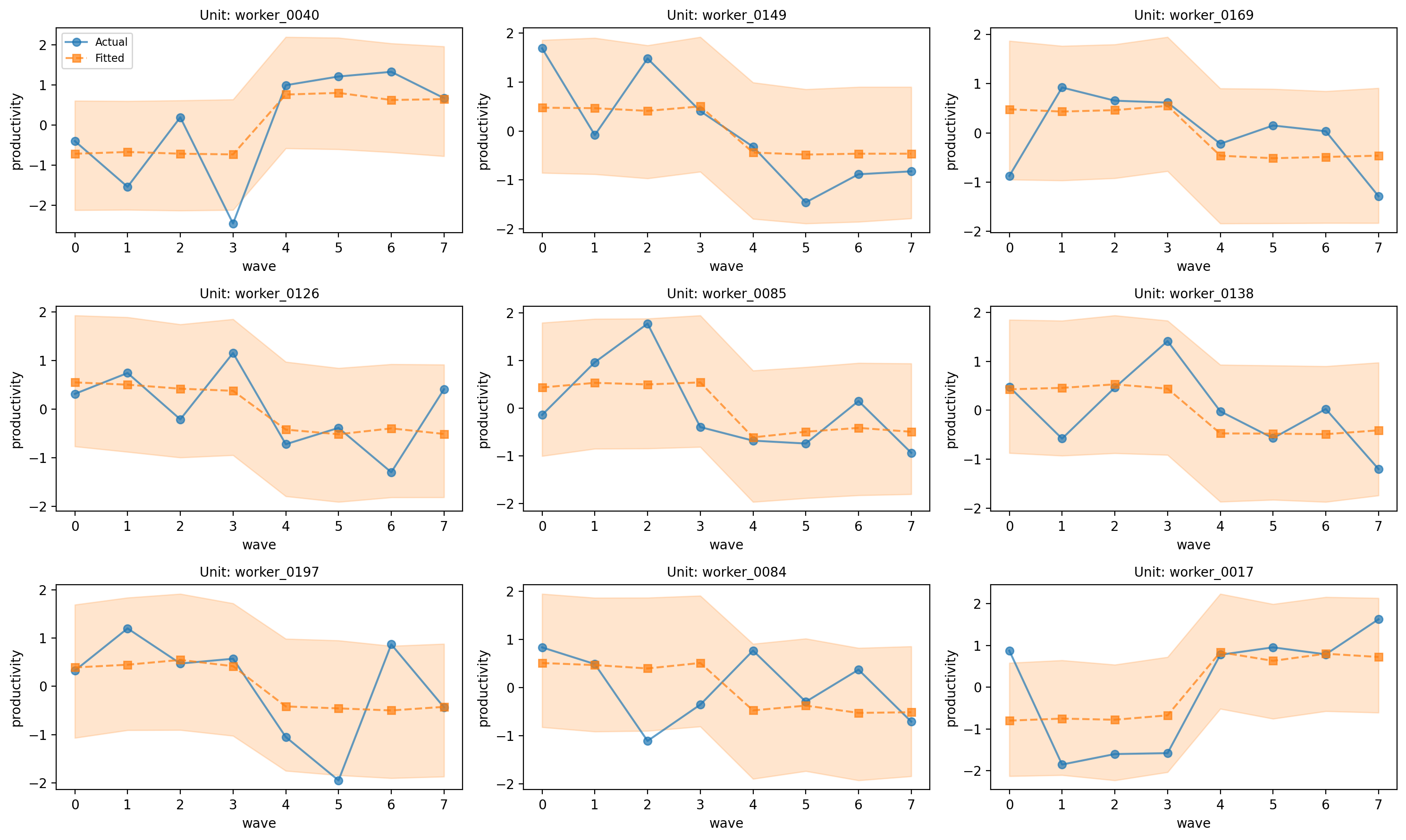
../_images/73b885fcb3836dfc0894acf395cac62e71dc0d6482c7c83e410ffc7e49b2b9d3.png

Figure (worker trajectories). Sample of worker-level productivity trajectories from the two-way FE model; observed vs predicted. Here the shaded band is a 94% posterior predictive HDI (interval_type="predictive"), which includes both parameter uncertainty and observation-level noise (y_hat). Adjust width with hdi_prob in plot_trajectories(...).

Let’s check some model diagnostics.

# Residuals vs fitted
fig, ax = result_states.plot_residuals(kind="scatter")
plt.tight_layout()
plt.show()

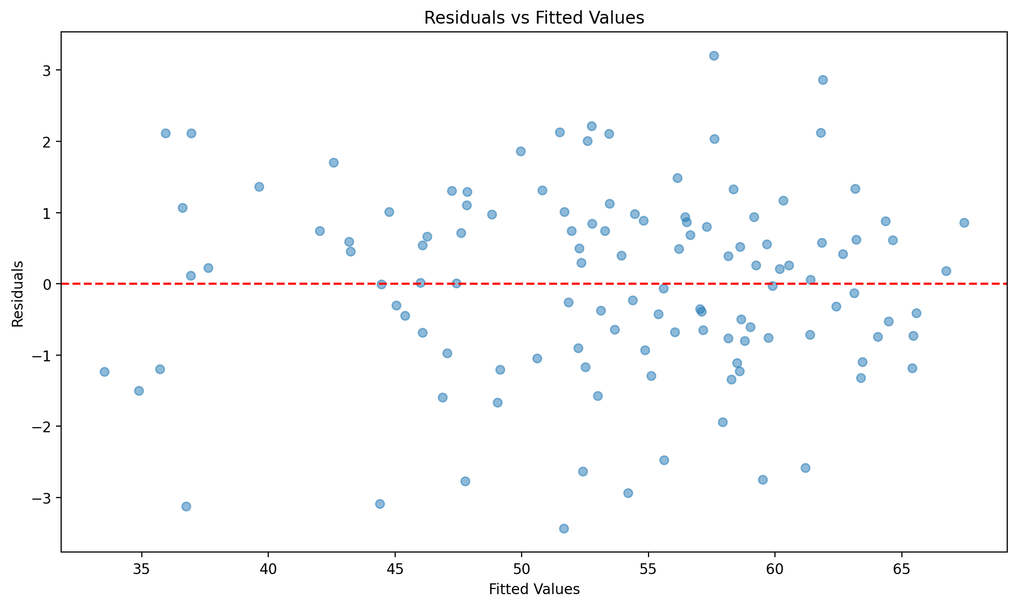
../_images/1cb7c8816dd40f600c3b6a9f5946ad04288a1ff5d28cc7db50a3d66774cad9b8.png

Figure (residuals vs fitted). Residuals from the state two-way FE model plotted against fitted values; used to check homoscedasticity and pattern in errors.

# Distribution of residuals
fig, ax = result_states.plot_residuals(kind="histogram")
plt.tight_layout()
plt.show()

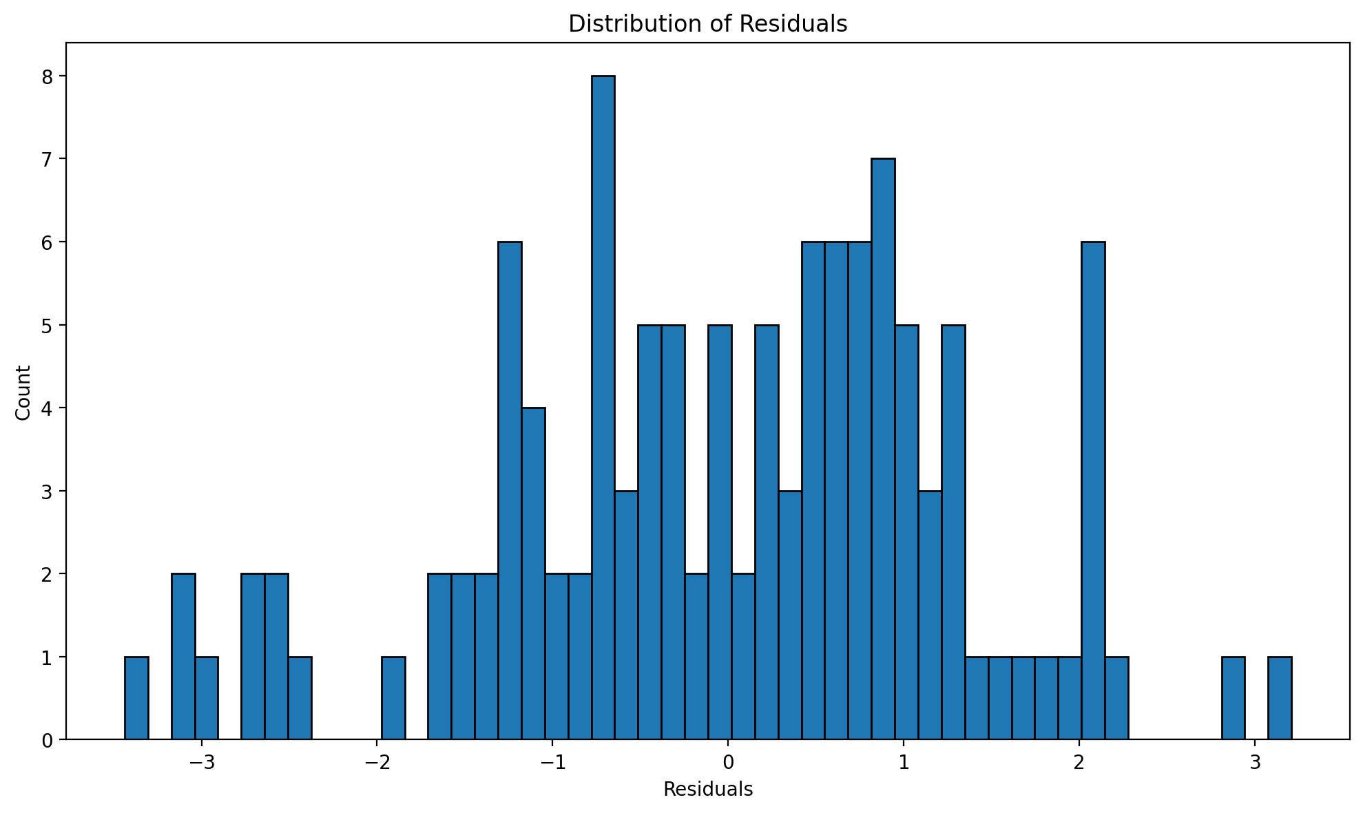
../_images/f16b4b56e467beacdf8ffc5056e177ed36c7227327965dc70d2d54e8262a6d20.png

Figure (residual distribution). Histogram of residuals from the state two-way FE model; used to assess normality of the error term.

# Q-Q plot
fig, ax = result_states.plot_residuals(kind="qq")
plt.tight_layout()
plt.show()

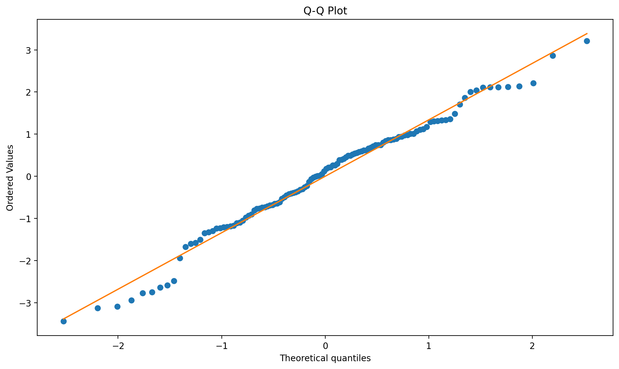
../_images/c2d9ad25ae1e97b1221601bae5b5fc8b26ac7952e2fdb52bb8ed5b2089d95449.png

Figure (Q–Q plot). Quantile-quantile plot of residuals vs theoretical normal; used to check normality of the error distribution.

Summary#

Key takeaways

Panel data = same units over time; fixed effects use this structure to control for unobserved unit and/or time confounders.
Unit FE removes time-invariant unit confounders; time FE removes common period shocks; two-way FE does both (and underlies DiD).
FE requires no time-varying confounders, strict exogeneity, and within-unit variation in treatment.
Demeaning and dummy-variable (unpooled) FE give the same treatment-effect estimate; use demeaning for large N.
FE cannot remove confounders that vary in both dimensions or reverse causality.

When to use fixed effects#

✅ Use Panel Fixed Effects when:

You have repeated observations on the same units
You suspect time-invariant unobserved confounders
Your treatment varies within units over time
You believe there are no time-varying confounders

❌ Don’t use when:

You only have cross-sectional data
Your treatment is time-invariant (it gets differenced out!)
There are likely time-varying confounders
Outcomes feed back into future treatment

Choosing Your Fixed Effects Specification#

Use this guide to select the appropriate fixed effects for your analysis:

Scenario	Recommended FE	Rationale
Units differ in time-invariant ways only	Unit FE only	Controls for unit heterogeneity; preserves time variation
All units experience common shocks each period	Time FE only	Controls for period effects; preserves cross-sectional variation
Both unit heterogeneity AND common time trends	Two-way FE	Controls for both; standard for DiD-style analyses
Time effects already captured by covariates	Unit FE only	Avoid over-controlling
Treatment is staggered across units	Two-way FE	Essential for valid DiD interpretation

Key Considerations

More FE is not always better: Adding fixed effects removes variation that could be useful for identification. Over-controlling can increase standard errors and even introduce bias.
Think about your DAG: What confounders exist? Are they time-invariant (unit FE), common across units (time FE), or both?
Treatment variation matters:
- If treatment only varies across units (not time), unit FE will absorb all treatment variation!
- If treatment only varies over time (not units), time FE will absorb all treatment variation!
Test sensitivity: When in doubt, run both one-way and two-way FE. If results differ substantially, investigate why.

Dummies vs Within#

Criterion	Dummies	Within
When	Small N (< 100)	Large N (100+)
Pros	Individual unit effects	Scales to large N
Cons	Doesn’t scale	Can’t estimate individual effects
Formula	`y ~ C(unit) + X`	`y ~ X`

Limitations and Caveats#

Before concluding, let’s be explicit about what fixed effects cannot do:

1. Cannot Remove Time-Varying Confounders: As demonstrated in our failure example, if unobserved factors change over time and affect both treatment and outcome, fixed effects will be biased. This is the most common limitation.
1. Cannot Solve Reverse Causality: If the outcome affects future treatment (feedback), fixed effects estimates are biased. Example: if poor sales cause firms to adopt new technology, we cannot estimate the effect of technology on sales using FE.
1. Removes Time-Invariant Variation: Fixed effects identifies effects from within-unit variation only. If your treatment barely varies within units, you have limited identifying variation and imprecise estimates.
1. Assumes Common Time Effects (Two-Way FE): With time fixed effects, you assume all units would follow parallel trends absent treatment. This may not hold if different units have different trajectories.

References#

[1]

Scott Cunningham. Causal inference: The mixtape. Yale university press, 2021.

[2]

Nick Huntington-Klein. The effect: An introduction to research design and causality. Chapman and Hall/CRC, 2021.

[3]

Jeffrey M Wooldridge. Econometric Analysis of Cross Section and Panel Data. MIT Press, 2nd edition, 2010.

[4] (1,2)

Kosuke Imai and In Song Kim. When should we use unit fixed effects regression models for causal inference with longitudinal data? American Journal of Political Science, 63(2):467–490, 2019.

[5]

Clément de Chaisemartin and Xavier D'Haultfœuille. Two-way fixed effects estimators with heterogeneous treatment effects. American Economic Review, 110(9):2964–2996, 2020.